Dates in Google Sheets are internally stored as numbers and the value is equal to the number of days since 30th December 1899, midnight. The time values are stored as a fractional number.
For instance, if the date in a cell is Jan 1 1990, Google Sheet will store the cell value as 2. If the date has a time component, say Jan 1 1900 6 PM, the internal date value will be 2.75.
The date and time values in Google Sheets are commonly displayed in the dd/mm/yyyy format, depending on your Spreadsheet locale, but this display format can be easily customized using the built-in TEXT function.
For instance, a date like 15/10/2021 can be displayed as Oct 15 2021 or in a long format like Friday, October 15 2021 or you may extract the time component and display it as 03:52 PM.

Convert Date Formats in Google Sheets
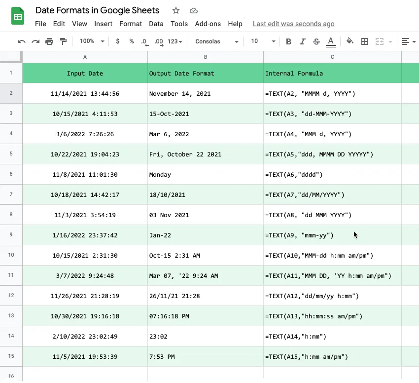
The TEXT function of Google Sheets allows to convert the date and time values in a sheet to a different format. It takes two parameters:
- The date or time value to be converted.
- The preferred format to convert the date or time value to.
=TEXT(A1, "MMMM d, YYYY")Here are some sample date formats that you can use in the second parameter of the TEXT function:
| Date and Time Pattern | Result |
|---|---|
| MMMM d, YYYY | October 21, 2021 |
| dd-MMM-YYYY | 08-Dec-2021 |
| MMM d, YYYY | Dec 3, 2021 |
| dd, MMMM DD YYYYY | Tue, October 19 2021 |
| ddd | Tuesday |
| d/MM/YYYY | 30/11/2021 |
| dd MMM YYYY | 06 Feb 2022 |
| mmm-yy | Oct-21 |
| dd/mm/yy h | 22/10/21 22 |
| hh:mm am/pm | 01:11 PM |
| h | 14 |
| h am/pm | 9 PM |
| MMM-dd h am/pm | Oct-20 10 PM |
| MMM DD, ‘YY h am/pm | Oct 31, ‘21 10 AM |
You can view the complete list in this Google Sheet.
Repeated Pattern in Custom Date Formats
The placeholders (like d, m or y) have different meanings depending on the number of pattern letters.
For instance, if the input date is October 5, the format code d will display the day of the month as 5 but if the format code is dd it will display zero-padded value as 05. If the format code is ddd, the result is an abbreviated day of the week Tue but if the format code is dddd, the full day of the week as Tuesday gets displayed.
Similarly, for the month placeholder, mm will display the zero-padded numerical value but mmm and mmmm will display the abbreviated and full month name respectively.
Date Formats with Array Formulas
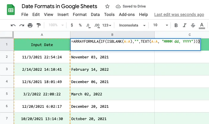
If you have a date column in Google Sheets and you want to display the date in a different format, you can use an array formula in a new column to convert the dates.
Assuming that the date column is in cell A1, you can use the following array formula in the first cell of an empty column to display the same date and time value but in a different format.
=ARRAYFORMULA(
  IF(ROW(A:A)=1,"New Date Format",
  IF(ISBLANK(A:A),"",TEXT(A:A, "MMMM dd, YYYY"))))
This can be very handy for Google Sheets that are storing Google Form responses. Google Sheet will always show the response timestamp in your locale but you can add a new column to display the date and time in a different format.
Also see: Google Sheets Formulas for Google Forms


