How to compare columns in Google Sheets and highlight cell values that are in one column but missing in another column.

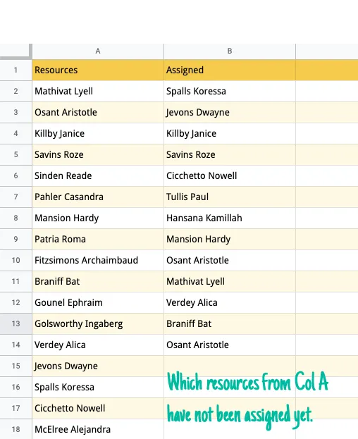
A small business maintains their staff roster in a simple Google Sheet - the column A of the sheet contains a list of all employee names and column B contains a list of employees who have been assigned to a project.

The immediate task is to identify staff members who are part of the organization but have not been assigned any project yet. In other words, the manager needs to figure out all employee names from column A who are not preset in column B.

There are two ways to solve this problem - visually and through formulas.

Using Visual Formatting

The first option would be to highlight cells in column A that are missing in column B.

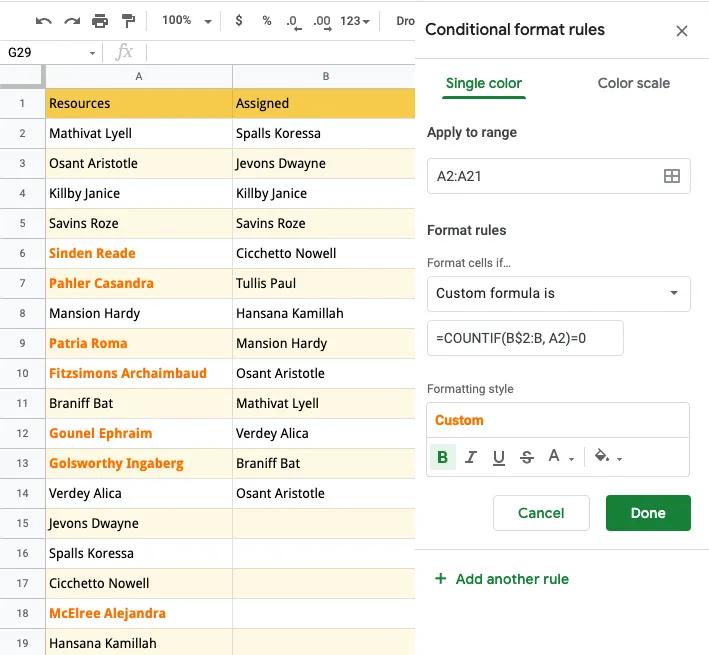
Inside the Google Sheet, go to the Format menu and choose conditional formatting. Here select A2:A for the range field, choose Custom Formula from the Format Cells If dropdown and paste the formula:

=COUNTIF(B$2:B, A2)=0

The COUNTIF function will essentially count the occurrence of each item in Column A against the range of cells in Column B. If the count for an item in Column A is 0, it means that the cell value is not present in column B and the cell is highlighted with a different background color.

Find Missing Items in Another Column

The next approach uses Google Sheet formulas to create a list of items that are in Column A but missing in Column B.

We’ll make use of the FILTER function that, as the name suggests, returns only a filtered version of a range that meets a specific criteria. In our case, the criteria is similar to the one that we used in the visual formatting section.

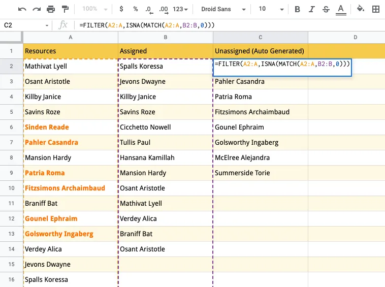
Go to column C (or any blank column) and enter this formula in the first empty cell.

=FILTER(A2:A,ISNA(MATCH(A2:A,B2:B,0)))

The MATCH function returns the position of items in Column A in the range associated with Column B and it returns #N/A if the values is not found. When the result is used with ISNA, it returns true only when the match is not found.

Using Google Query Language

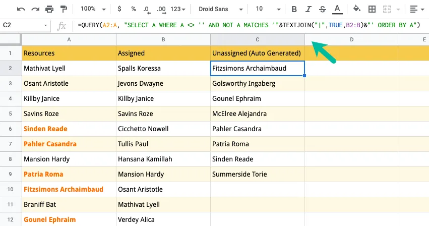
SQL geeks may also use the Google Query Language, we are used it with D3.js visualization, to print the list of names that are in Column B but not in Column B.

=QUERY(A2:A,
   "SELECT A WHERE A <> ''
    AND NOT A MATCHES '"&TEXTJOIN("|",TRUE,B2:B)&"'
    ORDER BY A")

The matches operator in the where clause does a regex comparison and the order by clause in the query will automatically sort the output alphabetically.