When someone submits a new Google Form response, the form answers are automaticaly added as a new row in the Google Sheet that is linked to the form. The only problem here is that Google Forms will not add any formatting or styles to the new row that you may have applied to the previous rows of the sheet.
Let me illustrate this with an example.
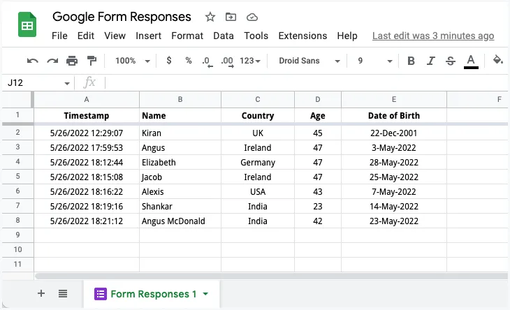
Here’s a screenshot of a Google Sheet that is storing Google Form responses. I’ve changed the default font family to Droid Sans, center-aligned the Country and Age column and also applied a different date format to the Date of Birth column.

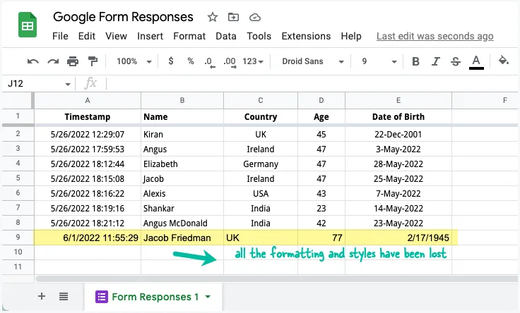
The formatting looks good but as soon as a new Google Form submissions is received, the new response row appended to the Google Sheet will lose all the formatting applied to the previous rows.
As you can see in the screenshot below, the cell alignment is not preserved, the custom date formats are ignored and so is the default font size and font family.

Auto Format New Rows in Google Sheets
Since there’s no way for us to override this Google Forms behavior, we can take the help of Google Apps Script to automatically format new rows in Google Sheets that are added through Google Forms.
To get started, open the Google Sheet and format the last row with the styles that you would like to apply to incoming form responses. Please ensure that there is at least one form response in the Google Sheet where you can apply the desired formatting that you want to be applied to new rows.
Add Google Apps Script to Google Sheet
Next, go to Extensions > Apps Script menu inside Google Sheets and copy-paste the Google Script below.
/**
 * @OnlyCurrentDoc
 */

const formatRowOnFormSubmit = formEvent => {
  try {
    const { range } = formEvent || {};
    if (!range) throw new Error("This function should only be triggered by form submissions");

    const sheet = range.getSheet();
    const currentRow = range.getRowIndex();
    const endColumn = sheet.getLastColumn();

    // Skip formatting if this is the first or second row
    if (currentRow <= 2) return;

    // Copy formatting from previous row to new row
    const sourceRange = sheet.getRange(currentRow - 1, 1, 1, endColumn);
    sourceRange.copyFormatToRange(sheet, 1, endColumn, currentRow, currentRow);
  } catch (error) {
    console.error(`Error formatting new response: ${error.message}`);
  }
};
Save the script. Next, we’ll create an onFormSubmit trigger inside the Google Sheet that will execute the formatRowOnFormSubmit function whenever a new form is submitted. This trigger will take whatever formatting that has been applied to the previous row and apply that to the current row.
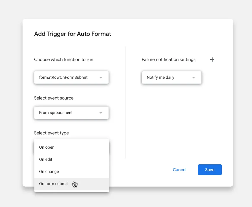
To create the trigger, go to the Triggers section in the sidebar and click + Add Trigger. Under the Event type dropdown, select On form submit and save the trigger. That’s it!

A previous version of the script used the
copyTomethod to copy formatting. While this approach works, the currentcopyFormatToRangemethod is more efficient as it’s specifically designed for copying only formatting between ranges.
const targetRange = sheet.getRange(currentRow, 1, 1, endColumn);
sourceRange.copyTo(targetRange, SpreadsheetApp.CopyPasteType.PASTE_FORMAT);
Conditional Formatting in Google Sheets
Learn more about conditional formatting in Google Sheets that allows you to apply automatic formatting to cells in spreadsheets that meet certain criteria.
Also see: Automate Google Forms through Workflows


