How to use the Index and Vlookup functions in Google Sheets with Match and ArrayFormula to lookup product prices that are listed as a table in the spreadsheet.

You run a coffee shop and you are looking for a spreadsheet formula to quickly look up prices of the product that your customer has ordered. You have the price matrix stored in a Google Sheet with the names of beverages in one column and the quantity-wise prices in the adjacent columns.

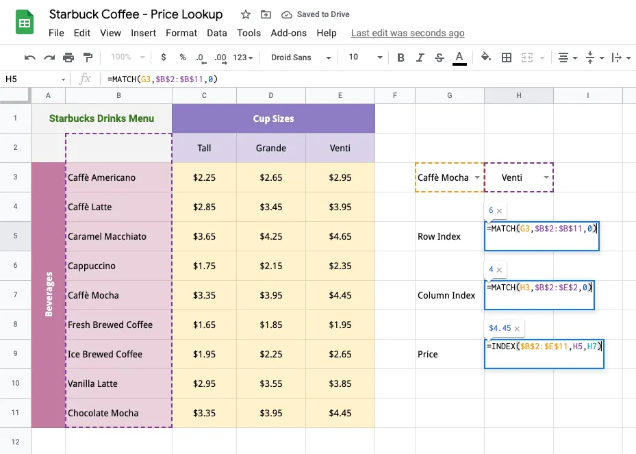
When a customer selects their favorite beverage and the cup size, you can use the MATCH function to find the relative position of the column and row in the price table that matches the selected beverage and quantity. Next, use the INDEX function to find the actual price of the beverage in the selected quantity.

In our Starbuck Coffee example, the coffee prices are stored in the range B2:B11. The customer’s beverage name (Caffè Mocha in this example) is stored in the cell G3. The following MATCH function will return the relative position of the selected beverage from the list of beverages.

=MATCH(G3, $B$2:$B$11, 0)

The third parameter of the MATCH function is set to 0 since we want the exact match and our price list is not sorted.

Similarly, the next MATCH function will return the relative position of the column that contains the price of the beverage based on the selected quantity. The cup sizes are stored in the range C2:E2. The selected cup size is stored in the cell H3.

=MATCH(H3, $B$2:$E$2, 0)

Now that we know the relative row and column position of the price value we are looking for, we can use the INDEX function to find the actual price from the table.

=INDEX($B$2:$E$11, H5, H7)

Use Vlookup with ArrayFormula and Match

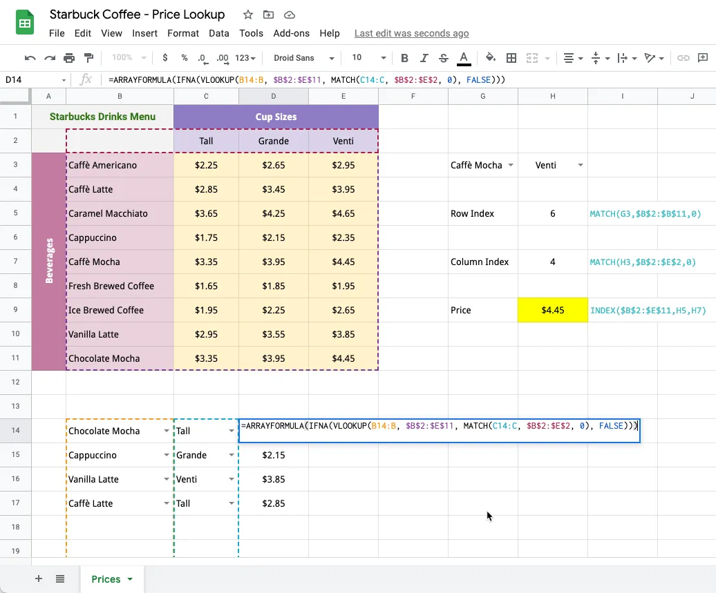
For the next example, we have a customer order that contains multiple beverages, one per row. We want to find the price of each beverage and the total price of the order. Array Formulas will be a perfect fit here since we want to extend the same formula to all rows of the spreadsheet.

However, we’ll have to revisit our approach since the INDEX function used in the previous example cannot be used with Array Formulas as it cannot return multiple values. We’ll replace INDEX with a similar VLOOKUP function and combine it with the MATCH function to perform a two-way lookup (find the beverage by name and then look for the specific cup size).

The VLOOKUP function syntax, in simple English, is:

=VLOOKUP(
  What you want to look for (beverage name),
  Where you want to look for it (price table range),
  The column number containing the matching value (chosen cup size),
  Return an approximate or exact match (True or False)
)

The function will look for the beverage name in the specified price range (B2:E11) and, from the matching row, return the value of the cell in the column that corresponds to selected cup size.

The price range is not sorted so we will put FALSE for the fourth parameter.

The MATCH function will return the relative position of the column that contains the price of the selected quantity of the matching beverage:

=MATCH(
  What are you looking for (cup size),
  Where are you looking for it (cup size header range),
  0 if you want to find the exact value (default is 1)
)

If a row doesn’t contain the beverage name, the formula will return #N/A and thus we wrap the value in IFNA to prevent the formula from returning any errors.

Our final formula will thus look like:

=ARRAYFORMULA(IFNA(VLOOKUP(B14:B, $B$2:$E$11, MATCH(C14:C, $B$2:$E$2, 0), FALSE)))

Download the Excel file - Price Lookup Sheet